プーリング・データとパネル・データ#
import numpy as np
import pandas as pd
import statsmodels.formula.api as smf
import wooldridge

from scipy.stats import t

# 警告メッセージを非表示
import warnings
warnings.filterwarnings("ignore")
説明#
独立に分布したプーリング・データ(independently distributed pooling data)とパネル・データ(panel data)を考える。両方とも横断面データと時系列データの両方の特徴を兼ね備えたデータである。
独立に分布したプーリング・データには以下の特徴がある。
ある期間(例えば,2000年から2010年の間)に期間毎無作為に観察単位(例えば,消費者や企業)が抽出される。従って,時間(年次データであれば年)が違えば観察単位は変化する。
時間の変化により必ずしも同一分布とはならない(即ち,分布は時間によって変化するかも知れない)。
日本の統計の例に労働力調査がある。
<プーリング・データを使う利点>
横断データと比べるとデータ数が増えるため,より正確な推定量や検定統計量を得ることが可能となる。
時間軸にそって独立した分布から標本を抽出するため,誤差項に自己相関はない。
パネル・データには以下の特徴がある。
初期時点で無作為に観察単位(例えば,消費者や企業)を抽出し,同じ観測単位を時間軸に沿って観測して集めたデータである。
観測単位が同じであることが独立に分布したプーリング・データとの違いである。
<パネル・データを使う意義>
例として,各都道府県で行われた公共支出が県内の雇用に与える影響を推定したいとしよう。
観察単位:47都道府県 \(i=1,2,...,47\)
時系列範囲:2000~2020年 \(t=2000,2001,...,2020\)
変数:県内の雇用(\(L\)),公共支出(\(G\)),\(x\)は「その他の変数」
47都道府県と時間の2次元データとなっているため,次の推定方法が考えられる。
年別に横断面データとしてクロス・セクション分析行う。
\[y_i = \beta_{0} + \beta_{1} G_i + \beta_{2}x_i + u_i\]しかし,それぞれの推定は20年間の間に起こる要因の変化の効果を無視することになり,公的支出の動的な側面を捉えていない。
47都道府県別に時系列の推定を行う。
\[y_t = \beta_{0} + \beta_{1} G_t + \beta_{2}x_t+ u_t\]しかし,それぞれの推定は同じ日本の地域でありながら他の都道府県の影響を無視することになる。
このように2次元のデータの1つの軸に沿ったデータだけを使うと何らかの影響を無視することになりうる。換言すると,パネル・データを使い異なる観察単位の動的なデータから得る情報を有効に使うことにより,より正確な推定量や検定統計量を得ることができることになる。
独立に分布したプーリング・データ#
このタイプのデータ扱う上で注意する点:
時系列の変数があるにも関わらず,被説明変数と少なくとも一部の説明変数とは時間不変の関係にあると暗に仮定することになる。
時系列の要素があるため,変数は必ずしも同一分布から抽出さる訳ではない。例えば,多くの経済で賃金と教育水準の分布は変化していると考える方が妥当である。この問題に対処するために時間ダミーを使うことになる。
CPS78_85のデータを使い推定方法を説明する。
# データの読み込み
cps = wooldridge.data('cps78_85')
# データの内容の確認
wooldridge.data('cps78_85', description=True)
name of dataset: cps78_85
no of variables: 15
no of observations: 1084

+----------+-----------------------+
| variable | label                 |
+----------+-----------------------+
| educ     | years of schooling    |
| south    | =1 if live in south   |
| nonwhite | =1 if nonwhite        |
| female   | =1 if female          |
| married  | =1 if married         |
| exper    | age - educ - 6        |
| expersq  | exper^2               |
| union    | =1 if belong to union |
| lwage    | log hourly wage       |
| age      | in years              |
| year     | 78 or 85              |
| y85      | =1 if year == 85      |
| y85fem   | y85*female            |
| y85educ  | y85*educ              |
| y85union | y85*union             |
+----------+-----------------------+

Professor Henry Farber, now at Princeton University, compiled these
data from the 1978 and 1985 Current Population Surveys. Professor
Farber kindly provided these data when we were colleagues at MIT.
このデータセットには1978年と1985年の変数があり,ダミー変数に次のものが含まれている。
y85:1985年の時間ダミー変数female:男女のダミー変数union:労働組合員かどうかのダミー変数
これを使い,賃金と教育の関係を検証する。
# 回帰分析

formula = 'lwage ~ y85 + educ + female + \
                   y85:educ + y85:female + \
                   exper + I((exper**2)/100) + union'

result = smf.ols(formula, cps).fit()
(コメント)
y85 + educ + female + y85:educ + y85:femaleの部分は長いのでy85*(educ+female)と省略して記述しても結果は同じ。lwageは名目賃金の対数の値である。この場合,実質賃金を考える方が自然なため,インフレの影響を取り除く必要がある。1978年と1985年の消費者物価指数をそれぞれ\(p_{78}\)と\(p_{85}\)とすると,その比率\(P\equiv p_{85}/p_{78}\)がその間のインフレの影響を捉える変数と考える。\(P\)を使い1985年の賃金を次式に従って実質化できる。\[ \ln\left(\text{実質賃金}_{85}\right) = \ln\left(\frac{\text{名目賃金}_{85}}{P}\right) = \ln\left(\text{名目賃金}_{85}\right)-\ln(P) = \text{85年のlwage}- \ln(P) \]この式から\(\ln(P)\)は回帰式の右辺の定数項に含まれることがわかる。即ち,上の式を変えることなく
educの係数は実質賃金で測った教育の収益率,femaleは実質賃金での男女賃金格差と解釈できる。
print(result.summary().tables[1])
=========================================================================================
                            coef    std err          t      P>|t|      [0.025      0.975]
-----------------------------------------------------------------------------------------
Intercept                 0.4589      0.093      4.911      0.000       0.276       0.642
y85                       0.1178      0.124      0.952      0.341      -0.125       0.361
educ                      0.0747      0.007     11.192      0.000       0.062       0.088
female                   -0.3167      0.037     -8.648      0.000      -0.389      -0.245
y85:educ                  0.0185      0.009      1.974      0.049       0.000       0.037
y85:female                0.0851      0.051      1.658      0.098      -0.016       0.186
exper                     0.0296      0.004      8.293      0.000       0.023       0.037
I((exper ** 2) / 100)    -0.0399      0.008     -5.151      0.000      -0.055      -0.025
union                     0.2021      0.030      6.672      0.000       0.143       0.262
=========================================================================================
教育の収益率
educの係数0.0747が1978年における教育1年の収益率(約7.5%)。統計的有意性は非常に高い(p-value=0)y85:educの係数0.0185は1978年と1985年の値の差を表している。1985年の収益率は1.85%高く,5%水準で帰無仮説(1978年と1985年の収益率は同じ)を棄却できる。1985年の1年間の収益率は0.0747+0.0185=0.0932である(約9.3%)。
男女間の賃金格差
femaleの係数-0.3167は1978年における値。即ち,女性の賃金は男性より約32%低く,統計的有意性は非常に高い(p値=0)。y85:femaleの係数0.0851は1978年と1985年の値の差を表しており,1985年の賃金格差は約8.5%改善したことを意味する。y85:femaleのp値0.098は両側検定であり,10%水準で帰無仮説(賃金格差は変化していない)を棄却できるが,5%水準では棄却できない。一方,
y85:femaleは正の値であり,女性の賃金の改善が統計的有意かどうかが問題になる。この点を考慮し片側検定をおこなう。\(H_0\):
y85:femaleの係数 \(=0\)\(H_a\):
y85:femaleの係数 \(>0\)
t_value = result.tvalues['y85:female']  # y85:femaleのt値

dof = result.df_resid  # 自由度 n-k-1
scipy.statsを使い計算する。
1-t.cdf(t_value, dof) # p値の計算
0.04884060330173612
片側検定では,5%水準で帰無仮説を棄却できる。
プーリング・データの応用:差分の差分析#
説明#
差分の差分析(Difference-in-Differences; DiD)を使うとプーリング・データを使い政策の効果を検証できる。
<基本的な考え>
例として,ゴミ焼却場の建築が近隣住宅価格に与える影響を考える。
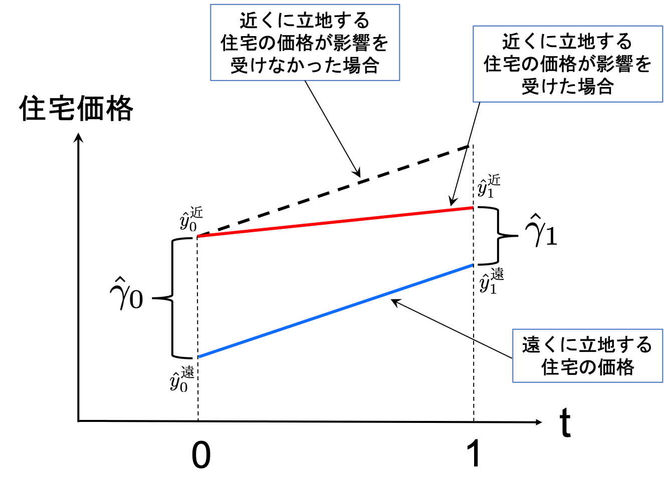
t=0:政策実施前の年t=1:政策実施後の年D:住宅がゴミ焼却場の近くであれば1,そうでなければ0(距離のダミー変数)y:住宅価格仮定:ゴミ焼却場が建設されなかったとしたら,データにある全ての住宅価格は同じ率で増加していただろう。
次式を使って政策実施前と後それぞれで推定
\[y_t = \alpha_t + \gamma_t D + u\qquad t=0,1\]\(\hat{y}_0^{\text{遠}}=\hat{\alpha}_0\):政策実施前の遠くに立地する住宅価格の平均
\(\hat{y}_0^{\text{近}}=\hat{\alpha}_0+\hat{\gamma}_0\):政策実施前の近くに立地する住宅価格の平均
\(\hat{\gamma}_0\):政策実施前の遠くと近くに立地する住宅価格の差
\(\hat{y}_1^{\text{遠}}=\hat{\alpha}_1\):政策実施後の遠くに立地する住宅価格の平均
\(\hat{y}_1^{\text{近}}=\hat{\alpha}_1+\hat{\gamma}_1\):政策実施後の近くに立地する住宅価格の平均
\(\hat{\gamma}_1\):政策実施後の遠くと近くに立地する住宅価格の差
解釈(下の図を参考に):
\(\hat{\gamma}_0\)は政策実施前の住宅価格の差を示す。
\(\hat{\gamma}_1\)は政策実施後の住宅価格の差を示す。
\(\left(\hat{\gamma}_1-\hat{\gamma}_0\right)\)は政策実施後と前の住宅価格の差の差を示す。この「差の差」の変化で近くに立地する住宅価格の変化を考えることができる。もしこの差の差が
0であれば(即ち,差は同じだった),住宅価格は影響を受けなかったと解釈できる。もしこの差がマイナスであれば(即ち,差に違いが生じた)近くに立地する住宅の価格は減少してしたと考えられる。
上の議論から次のことが分かる。
住宅価格の変化は上の図で示しているように次の「差の差」で捉えることができる。
\[\begin{split} \begin{align*} \hat{\gamma}_1^{\text{}}-\hat{\gamma}_0&=\hat{y}_1^{\text{近}}-\hat{y}_0^{\text{近}}-\left(\hat{\alpha}_1-\hat{\alpha}_0\right) \\ &=\left(\hat{y}_1^{\text{近}}-\hat{y}_0^{\text{近}}\right)-\left(\hat{y}_1^{\text{遠}}-\hat{y}_0^{\text{遠}}\right) \\ &=\left(\hat{y}_1^{\text{近}}-\hat{y}_1^{\text{遠}}\right)-\left(\hat{y}_0^{\text{近}}-\hat{y}_0^{\text{遠}}\right) \end{align*} \end{split}\]住宅価格の変化の間違った計算:
\(\hat{y}_1^{\text{近}}-\hat{y}_0^{\text{近}}=\left(\hat{\alpha}_1-\hat{\alpha}_0\right)+\left(\hat{\gamma}_1-\hat{\gamma}_0\right)\)
\(\left(\hat{\alpha}_1-\hat{\alpha}_0\right)\)は,ゴミ焼却場建設から影響を「受けない(仮定)」遠 い場所に立地する住宅価格が時間と共に変化する部分を捉えており,ゴミ焼却場建設と関係なく発生する価格変化である。この部分を取り除かなければ,ゴミ焼却場建設の効果の推定量にバイアスが発生する。
<DiD推定方法>
通常の
OLSを使うが,時間ダミー変数を導入する。T:t=0の場合は0,t=1の場合は1
推定式:
\[ y=\beta_0+\delta_0T + \beta_1D + \delta_1TD + u \]
<ダミー変数の値により4つのケースがある>
T=D=0の場合\[ y=\beta_0 + u \]\(\hat{y}_{0}^{\text{遠}}\equiv\hat{\beta}_0\):政策実施前の遠くに立地する住宅の平均価格
T=0 とD=1の場合\[ y=\beta_0 + \beta_1D + u \]\(\hat{y}_{0}^{\text{近}}\equiv\hat{\beta}_0+\hat{\beta}_1\):政策実施前の近くに立地する住宅の平均価格
T=1 とD=0の場合\[ y=\beta_0 + \delta_0T + u \]\(\hat{y}_{1}^{\text{遠}}\equiv\hat{\beta}_0+\hat{\delta}_0\):政策実施後の遠くに立地する住宅の平均価格
T=D=1の場合\[ y=\beta_0 + \delta_0T + \beta_1D + \delta_1TD + u \]\(\hat{y}_{1}^{\text{近}}\equiv\hat{\beta}_0+\hat{\delta}_0+\hat{\beta}_1+\hat{\delta}_1\):政策実施後の近くに立地する住宅の平均価格
ここでの関心事は\(\hat{\delta}_1\)の推定値(負かどうか)であり,その統計的優位性である。この定義を使うと次式が成立することが確認できる。
これは上で導出した式にある\(\hat{\gamma}_1^{\text{}}-\hat{\gamma}_0\)と同じである。
DiD推定#
keilmcのデータを使いゴミ焼却場建設の近隣住宅価格に対する効果を実際に推計する。
kielmc = wooldridge.data('kielmc')

wooldridge.data('kielmc', description=True)
name of dataset: kielmc
no of variables: 25
no of observations: 321

+----------+---------------------------------+
| variable | label                           |
+----------+---------------------------------+
| year     | 1978 or 1981                    |
| age      | age of house                    |
| agesq    | age^2                           |
| nbh      | neighborhood, 1-6               |
| cbd      | dist. to cent. bus. dstrct, ft. |
| intst    | dist. to interstate, ft.        |
| lintst   | log(intst)                      |
| price    | selling price                   |
| rooms    | # rooms in house                |
| area     | square footage of house         |
| land     | square footage lot              |
| baths    | # bathrooms                     |
| dist     | dist. from house to incin., ft. |
| ldist    | log(dist)                       |
| wind     | prc. time wind incin. to house  |
| lprice   | log(price)                      |
| y81      | =1 if year == 1981              |
| larea    | log(area)                       |
| lland    | log(land)                       |
| y81ldist | y81*ldist                       |
| lintstsq | lintst^2                        |
| nearinc  | =1 if dist <= 15840             |
| y81nrinc | y81*nearinc                     |
| rprice   | price, 1978 dollars             |
| lrprice  | log(rprice)                     |
+----------+---------------------------------+

K.A. Kiel and K.T. McClain (1995), “House Prices During Siting
Decision Stages: The Case of an Incinerator from Rumor Through
Operation,” Journal of Environmental Economics and Management 28,
241-255. Professor McClain kindly provided the data, of which I used
only a subset.
formula = 'rprice ~ nearinc + y81 + nearinc:y81'

result = smf.ols(formula, data=kielmc).fit()
(コメント)
右辺を
nearinc * y81と省略可能。
print(result.summary().tables[1])
===============================================================================
                  coef    std err          t      P>|t|      [0.025      0.975]
-------------------------------------------------------------------------------
Intercept    8.252e+04   2726.910     30.260      0.000    7.72e+04    8.79e+04
nearinc     -1.882e+04   4875.322     -3.861      0.000   -2.84e+04   -9232.293
y81          1.879e+04   4050.065      4.640      0.000    1.08e+04    2.68e+04
nearinc:y81 -1.186e+04   7456.646     -1.591      0.113   -2.65e+04    2806.867
===============================================================================
nearinc:y81の係数は約-11860であり,10%水準の両側検定でも帰無仮説(係数は0)を棄却できない。nearinc:y81は負の値であり住宅価格が減少したかを検証したい。従って,次の片側検定を行う。\(H_0\):
nearinc:y81の係数 \(=0\)\(H_a\):
nearinc:y81の係数 \(<0\)
t_value = result.tvalues['nearinc:y81']  # t値

dof = result.df_resid  # 自由度 n-k-1

t.cdf(t_value, dof)  # p値の計算
0.05629742034952766
片側検定では,10%水準で帰無仮説は棄却できるが,5%水準では棄却できない。負の効果のある程度の統計的有意性はあるようである。一方,上の回帰分析には次のことが言える。
左辺には住宅価格の対数を置く方が妥当ではないか。それにより,価格変化をパーセンテージ推計できると同時に,実質価格という解釈も成立する。
住宅価格に与える他の変数が欠落している可能性がある。
この2点を踏まえて,再度推定をおこなう。
まず,NumPyを使い住宅価格に対数をとり推計する。
formula_1 = 'np.log(rprice) ~ nearinc * y81'

result_1 = smf.ols(formula_1, data=kielmc).fit()

print(result_1.summary().tables[1])
===============================================================================
                  coef    std err          t      P>|t|      [0.025      0.975]
-------------------------------------------------------------------------------
Intercept      11.2854      0.031    369.839      0.000      11.225      11.345
nearinc        -0.3399      0.055     -6.231      0.000      -0.447      -0.233
y81             0.1931      0.045      4.261      0.000       0.104       0.282
nearinc:y81    -0.0626      0.083     -0.751      0.453      -0.227       0.102
===============================================================================
(結果)
特に
nearinc:y81の係数の統計的有意性が上昇したわけではない。
次に,住宅価格に影響を及ぼしそうな変数を追加する。
formula_2 = 'np.log(rprice) ~ nearinc * y81 + age + I(age**2) + \
            np.log(intst) + np.log(land) + np.log(area) + rooms + baths'

result_2 = smf.ols(formula_2, data=kielmc).fit()

print(result_2.summary().tables[1])
=================================================================================
                    coef    std err          t      P>|t|      [0.025      0.975]
---------------------------------------------------------------------------------
Intercept         7.6517      0.416     18.399      0.000       6.833       8.470
nearinc           0.0322      0.047      0.679      0.498      -0.061       0.126
y81               0.1621      0.028      5.687      0.000       0.106       0.218
nearinc:y81      -0.1315      0.052     -2.531      0.012      -0.234      -0.029
age              -0.0084      0.001     -5.924      0.000      -0.011      -0.006
I(age ** 2)    3.763e-05   8.67e-06      4.342      0.000    2.06e-05    5.47e-05
np.log(intst)    -0.0614      0.032     -1.950      0.052      -0.123       0.001
np.log(land)      0.0998      0.024      4.077      0.000       0.052       0.148
np.log(area)      0.3508      0.051      6.813      0.000       0.249       0.452
rooms             0.0473      0.017      2.732      0.007       0.013       0.081
baths             0.0943      0.028      3.400      0.001       0.040       0.149
=================================================================================
(結果)
nearinc:y81の係数は,住宅価格が13.1%下落したことを示している。p値はこの経済的効果が非常に有意にゼロではないことを示している。
パネル・データとその問題点#
パネル・データについて#
パネル・データを使い推定する場合,観察単位\(i\)と時間\(t\)の2つ次元を考慮した回帰式となる。説明を具体化するために,47都道府県での雇用に対する公共支出の効果を考えよう。
ここで
\(y_{it}\):都道府県\(i\)の\(t\)時点における雇用
\(x_{it}\):都道府県\(i\)の\(t\)時点における公共支出
\(\alpha_{it}\):回帰曲線の切片。
\(i\)がある(都道府県によって切片が異なる)理由:都道府県の間に存在しうる異質性を捉えている。
例えば,他県の公共支出からの影響を受けやすい(若しくは,受けにくい)県がある可能性がある。また,海に接している県や内陸の県では公共支出の効果は異なるかも知れない。また働き方や公共支出に対する県民特有の考え方や好みの違いもありうる。こういう要素は変化には時間が掛かり,推定期間内であれば一定と考えることができる。ありとあらゆる異質性が含まれるため,観察不可能と考えられる。
\(t\)がある理由:公共支出以外の理由で時間と共に雇用は変化するかもしれない。時間トレンドの効果を捉える。
都道府県特有の定数項は3つに分ける。
\(\beta_0\):共通の定数項
\(a_{i}\):都道府県別の定数項(観察不可能)
\(\delta_0D_t\):時間による切片の変化を捉えており,\(D_t\)は時間ダミー変数
\(D_0=0\)
\(D_1=1\)
\(u_{it}\):時間によって変化する観測不可能な誤差項(\(i\)と\(t\)に依存する誤差項であり,idiosyncratic errorsと呼ばれることがある)
仮定:\(\text{Cov}(x_{it},u_{it})=0\)
OLS推定の問題点#
\(a_i\)は観察不可能なため,上の回帰式は次のように表すことができる。
ここで\(e_{it}\)は観察不可能な誤差項。
\(x_{it}\)と\(a_i\)とが相関する場合,\(x_{it}\)と\(e_{it}\)は相関することになり,GM仮定4は成立しなくなる。
\[ \text{Cov}\left(x_{it}a_{it}\right)\neq 0\quad \Rightarrow\quad \text{Cov}\left(x_{it}e_{it}\right)\neq 0 \]即ち,\(\hat{\beta}_1\)は不偏性と一致性を失うことになる。
「異質性バイアス」と呼ばれるが,本質的には\(a_i\)の欠落変数バイアスである。
1階差分推定の準備:groupby#
パネル・データを使った推定方法として1階差分推定(First Differenced Estimator)があり,それを使い推定する。その前準備として変数の差分の作成方法について説明する。
DataFrameにはメソッドgroupbyがあり,これを使うとカテゴリー変数がある列に従って行をグループ分けしグループ毎の様々な計算が可能となる。具体的な例としてはGapminderを参照。ここではgroupbyを使い差分の変数の作り方を説明する。
例として使うデータを読み込む。
# url の設定
url = 'https://raw.githubusercontent.com/Haruyama-KobeU/Haruyama-KobeU.github.io/master/data/data4.csv'

# 読み込み
df = pd.read_csv(url)

df
| year | country | gdp | inv | con | pop | |
|---|---|---|---|---|---|---|
| 0 | 2000 | Australia | 90 | 30.0 | 50.0 | 10 |
| 1 | 2001 | Australia | 100 | 40.0 | 80.0 | 11 |
| 2 | 2002 | Australia | 120 | NaN | 70.0 | 16 |
| 3 | 2000 | Japan | 100 | 20.0 | 80.0 | 8 |
| 4 | 2001 | Japan | 95 | 25.0 | 70.0 | 9 |
| 5 | 2002 | Japan | 93 | 21.0 | 72.0 | 10 |
| 6 | 2000 | UK | 100 | 30.0 | 70.0 | 11 |
| 7 | 2001 | UK | 110 | 39.0 | 71.0 | 12 |
| 8 | 2002 | UK | 115 | 55.0 | NaN | 14 |
列countryがカテゴリー変数であり,3つの国がある。この列を使いグループ分けする。
まず前準備として,メソッド.sort_values()を使い列countryで昇順に並び替え,その後,列yearで昇順に並び替える。
(コメント)
以下のコードには.reset_index(drop=True)が追加されているが,これは行のインデックスを0,1,2,..と振り直すメソッドである。引数drop=Trueがなければ,元々あったインデックスが新たな列として追加される。試しに,最初からdfを読み直して.reset_index(drop=True)を省いて下のコードを実行してみよう。
df = df.sort_values(['country','year']).reset_index(drop=True)

df
| year | country | gdp | inv | con | pop | |
|---|---|---|---|---|---|---|
| 0 | 2000 | Australia | 90 | 30.0 | 50.0 | 10 |
| 1 | 2001 | Australia | 100 | 40.0 | 80.0 | 11 |
| 2 | 2002 | Australia | 120 | NaN | 70.0 | 16 |
| 3 | 2000 | Japan | 100 | 20.0 | 80.0 | 8 |
| 4 | 2001 | Japan | 95 | 25.0 | 70.0 | 9 |
| 5 | 2002 | Japan | 93 | 21.0 | 72.0 | 10 |
| 6 | 2000 | UK | 100 | 30.0 | 70.0 | 11 |
| 7 | 2001 | UK | 110 | 39.0 | 71.0 | 12 |
| 8 | 2002 | UK | 115 | 55.0 | NaN | 14 |
countryでグループ化したdf_groupを作成する。
df_group = df.groupby('country')

df_group
<pandas.core.groupby.generic.DataFrameGroupBy object at 0x11b1944a0>
このコードの出力が示すように,df_groupはDataFrameGroupByというクラス名のオブジェクト(データ型)であり,DataFrameとは異なる。これによりグループ別の計算が格段と容易になる。
例えば,次のコードを使いそれぞれの経済のgdpの平均を計算することができる。
df_group['gdp'].mean()
country
Australia    103.333333
Japan         96.000000
UK           108.333333
Name: gdp, dtype: float64
mean()はdf_groupに備わるメソッドである。他にも便利な使い方があるが,ここでは変数の差分の作りかを説明する。
df_groupにある変数の差分をとるためにメソッドdiff()を使う。
var = ['gdp', 'inv']

df_diff = df_group[var].diff()

df_diff
| gdp | inv | |
|---|---|---|
| 0 | NaN | NaN |
| 1 | 10.0 | 10.0 |
| 2 | 20.0 | NaN |
| 3 | NaN | NaN |
| 4 | -5.0 | 5.0 |
| 5 | -2.0 | -4.0 |
| 6 | NaN | NaN |
| 7 | 10.0 | 9.0 |
| 8 | 5.0 | 16.0 |
次にdfとdf_diffを横に結合する。
<方法1:pd.concat>
df_diffの列名を変更pd.concatを使い結合
df_diff_1 = df_diff.rename(columns={'gdp':'gdp_diff','inv':'inv_diff'})

df_diff_1
| gdp_diff | inv_diff | |
|---|---|---|
| 0 | NaN | NaN |
| 1 | 10.0 | 10.0 |
| 2 | 20.0 | NaN |
| 3 | NaN | NaN |
| 4 | -5.0 | 5.0 |
| 5 | -2.0 | -4.0 |
| 6 | NaN | NaN |
| 7 | 10.0 | 9.0 |
| 8 | 5.0 | 16.0 |
pd.concat([df, df_diff_1], axis='columns')
| year | country | gdp | inv | con | pop | gdp_diff | inv_diff | |
|---|---|---|---|---|---|---|---|---|
| 0 | 2000 | Australia | 90 | 30.0 | 50.0 | 10 | NaN | NaN |
| 1 | 2001 | Australia | 100 | 40.0 | 80.0 | 11 | 10.0 | 10.0 |
| 2 | 2002 | Australia | 120 | NaN | 70.0 | 16 | 20.0 | NaN |
| 3 | 2000 | Japan | 100 | 20.0 | 80.0 | 8 | NaN | NaN |
| 4 | 2001 | Japan | 95 | 25.0 | 70.0 | 9 | -5.0 | 5.0 |
| 5 | 2002 | Japan | 93 | 21.0 | 72.0 | 10 | -2.0 | -4.0 |
| 6 | 2000 | UK | 100 | 30.0 | 70.0 | 11 | NaN | NaN |
| 7 | 2001 | UK | 110 | 39.0 | 71.0 | 12 | 10.0 | 9.0 |
| 8 | 2002 | UK | 115 | 55.0 | NaN | 14 | 5.0 | 16.0 |
上のコードのaxis='columns'はaxis=1としてもOK。この方法は、dfとdf_diff_1の行の順序が同じという想定のもとで行っている。行の順番が同じでない場合や不明な場合は、次の方法が良いであろう。
<方法2:pd.merge>
dfとdf_diffを使い、方法1の2つのステップを1行で済ませる。次のコードでは3つの引数を指定している。
left_index=Truedfの行のインデックスに合わせて結合する。
right_index=Truedf_diffの行のインデックスに合わせて結合する。
suffixes=('', '_diff')左の引数
'':結合後,重複する左のDataFrameの列につける接尾辞(空の接尾辞)右の引数
'_diff':結合後,重複する右のDataFrameの列につける接尾辞
pd.merge(df, df_diff, left_index=True, right_index=True, suffixes=('', '_diff'))
| year | country | gdp | inv | con | pop | gdp_diff | inv_diff | |
|---|---|---|---|---|---|---|---|---|
| 0 | 2000 | Australia | 90 | 30.0 | 50.0 | 10 | NaN | NaN |
| 1 | 2001 | Australia | 100 | 40.0 | 80.0 | 11 | 10.0 | 10.0 |
| 2 | 2002 | Australia | 120 | NaN | 70.0 | 16 | 20.0 | NaN |
| 3 | 2000 | Japan | 100 | 20.0 | 80.0 | 8 | NaN | NaN |
| 4 | 2001 | Japan | 95 | 25.0 | 70.0 | 9 | -5.0 | 5.0 |
| 5 | 2002 | Japan | 93 | 21.0 | 72.0 | 10 | -2.0 | -4.0 |
| 6 | 2000 | UK | 100 | 30.0 | 70.0 | 11 | NaN | NaN |
| 7 | 2001 | UK | 110 | 39.0 | 71.0 | 12 | 10.0 | 9.0 |
| 8 | 2002 | UK | 115 | 55.0 | NaN | 14 | 5.0 | 16.0 |
dfを上書きしたい場合は,df=を付け加える。
1階差分推定#
説明#
異質性バイアスの一番簡単な解決方法が1階差分推定(First Differenced Estimator)である。考え方は非常に簡単である。次の1階差分を定義する。
\(\Delta y_{i}=y_{i1}-y_{i0}\)
\(\Delta D = D_{1}-D_0 =1-0= 1\)
\(\Delta x_{i}=x_{i1}-x_{i0}\)
\(\Delta e_{i}=e_{i1}-e_{i0}=a_i+u_{i1}-\left(a_i+u_{i0}\right)=\Delta u_{i}\)
\(a_i\)が削除される。
これらを使い,上の式の1階差分をとると次式を得る。
良い点
(仮定により)\(\Delta x_{i}\)と\(\Delta u_{i}\)は相関しないため,GM仮定4は満たされることになる。
悪い点
\(t=0\)のデータを使えなくなるため,標本の大きさが小さくなる。
期間内の説明変数\(\Delta x_i\)の変化が小さいと,不正確な推定になる(極端な場合,変化がないと推定不可能となる)。
<推定方法>
データから1階差分を計算し,statsmodelsを使いOLS推定すれば良い。以下ではパッケージwooldridgeにあるデータを使う。
推定:2期間の場合#
以下では
crime2のデータを使い説明する。このデータを使い,失業率が犯罪に負の影響を与えるかどうかを検証する。
データの読み込み。
crime2 = wooldridge.data('crime2')
変数の説明。
wooldridge.data('crime2', description=True)
name of dataset: crime2
no of variables: 34
no of observations: 92

+----------+----------------------------+
| variable | label                      |
+----------+----------------------------+
| pop      | population                 |
| crimes   | total number index crimes  |
| unem     | unemployment rate          |
| officers | number police officers     |
| pcinc    | per capita income          |
| west     | =1 if city in west         |
| nrtheast | =1 if city in NE           |
| south    | =1 if city in south        |
| year     | 82 or 87                   |
| area     | land area, square miles    |
| d87      | =1 if year = 87            |
| popden   | people per sq mile         |
| crmrte   | crimes per 1000 people     |
| offarea  | officers per sq mile       |
| lawexpc  | law enforce. expend. pc, $ |
| polpc    | police per 1000 people     |
| lpop     | log(pop)                   |
| loffic   | log(officers)              |
| lpcinc   | log(pcinc)                 |
| llawexpc | log(lawexpc)               |
| lpopden  | log(popden)                |
| lcrimes  | log(crimes)                |
| larea    | log(area)                  |
| lcrmrte  | log(crmrte)                |
| clcrimes | change in lcrimes          |
| clpop    | change in lpop             |
| clcrmrte | change in lcrmrte          |
| lpolpc   | log(polpc)                 |
| clpolpc  | change in lpolpc           |
| cllawexp | change in llawexp          |
| cunem    | change in unem             |
| clpopden | change in lpopden          |
| lcrmrt_1 | lcrmrte lagged             |
| ccrmrte  | change in crmrte           |
+----------+----------------------------+

These data were collected by David Dicicco, a former MSU
undergraduate, for a final project. They came from various issues of
the County and City Data Book, and are for the years 1982 and 1985.
Unfortunately, I do not have the list of cities.
興味がある変数
crmes:犯罪率(1000人当たり犯罪数)unem:失業率
(コメント)
データセットにはこの2つの変数の差分(cunemとccrmrte)も用意されているが,以下ではgroupbyを使って変数を作成する。
crime2.head()
| pop | crimes | unem | officers | pcinc | west | nrtheast | south | year | area | ... | clcrimes | clpop | clcrmrte | lpolpc | clpolpc | cllawexp | cunem | clpopden | lcrmrt_1 | ccrmrte | |
|---|---|---|---|---|---|---|---|---|---|---|---|---|---|---|---|---|---|---|---|---|---|
| 0 | 229528.0 | 17136.0 | 8.2 | 326 | 8532 | 1 | 0 | 0 | 82 | 44.599998 | ... | NaN | NaN | NaN | 0.350872 | NaN | NaN | NaN | NaN | NaN | NaN |
| 1 | 246815.0 | 17306.0 | 3.7 | 321 | 12155 | 1 | 0 | 0 | 87 | 44.599998 | ... | 0.009871 | 0.072614 | -0.062743 | 0.262802 | -0.08807 | 0.977952 | -4.5 | 0.072615 | 4.312912 | -4.540268 |
| 2 | 814054.0 | 75654.0 | 8.1 | 1621 | 7551 | 1 | 0 | 0 | 82 | 375.000000 | ... | NaN | NaN | NaN | 0.688772 | NaN | NaN | NaN | NaN | NaN | NaN |
| 3 | 933177.0 | 83960.0 | 5.4 | 1803 | 11363 | 1 | 0 | 0 | 87 | 375.000000 | ... | 0.104170 | 0.136568 | -0.032398 | 0.658612 | -0.03016 | 0.200762 | -2.7 | 0.136568 | 4.531899 | -2.962654 |
| 4 | 374974.0 | 31352.0 | 9.0 | 633 | 8343 | 1 | 0 | 0 | 82 | 49.799999 | ... | NaN | NaN | NaN | 0.523614 | NaN | NaN | NaN | NaN | NaN | NaN |
5 rows × 34 columns
このデータセットには,観察単位識別用の変数がない。しかし,行0と1が1つの地域のデータ,行2と3が別の地域のデータをなっていることがわかる(yearを見るとわかる)。まず観察単位識別用の列を作成する。
# 観察単位の数
n = len(crime2)/2

# 観察単位ID用のリスト作成 [1,2,3,4....]
lst = [i for i in range(1,int(n)+1)]

# 観察単位ID用のリスト作成 [1,1,2,2,3,3,4,4....]
country_list = pd.Series(lst).repeat(2).to_list()
country_listの説明:
Seriesのメソッドrepeat(2)はlstの要素を2回リピートするSeriesを生成する。to_list()はSeriesをリストに変換するメソッド。
データセットに列countyを追加し確認する。
crime2['county'] = country_list  # 追加

crime2.loc[:,['county','year']].head()  # 確認
| county | year | |
|---|---|---|
| 0 | 1 | 82 |
| 1 | 1 | 87 |
| 2 | 2 | 82 |
| 3 | 2 | 87 |
| 4 | 3 | 82 |
unemとcrmrteの差分を求める。
var = ['unem', 'crmrte']  # groupbyで差分を取る列の指定

names = {'unem':'unem_diff', 'crmrte':'crmrte_diff'}  # 差分の列のラベル

crime2_diff = crime2.groupby('county')[var].diff().rename(columns=names)

crime2_diff.head()
| unem_diff | crmrte_diff | |
|---|---|---|
| 0 | NaN | NaN |
| 1 | -4.5 | -4.540268 |
| 2 | NaN | NaN |
| 3 | -2.7 | -2.962654 |
| 4 | NaN | NaN |
crime2_diffを使って回帰分析をおこなう。
(コメント)
以下の計算ではNaNは自動的に無視される。
formula_1 = 'crmrte_diff ~ unem_diff'

result_1 = smf.ols(formula_1, crime2_diff).fit()

print(result_1.summary().tables[1])
==============================================================================
                 coef    std err          t      P>|t|      [0.025      0.975]
------------------------------------------------------------------------------
Intercept     15.4022      4.702      3.276      0.002       5.926      24.879
unem_diff      2.2180      0.878      2.527      0.015       0.449       3.987
==============================================================================
<結果>
失業率が1%増加すると,犯罪率は約2.2%上昇する。
この場合、微分を計算するのではなく、
unem_diffに1を代入して解釈する。
5%の水準で帰無仮説を棄却できる。
次の片側検定を行う
\(H_0\):
unemの係数 \(=0\)\(H_a\):
unemの係数 \(>0\)
t_value = result_1.tvalues['unem_diff']  # t値

dof = result_1.df_resid  # 自由度 n-k-1

1-t.cdf(t_value, dof)  # p値の計算
0.007594658874412463
片側検定では,1%水準で帰無仮説を棄却できる。
<参考1>
1階差分推定を使わずに直接OLS推定するとどうなるかを確かめてみる。
formula_ols_1 = 'crmrte ~ d87 + unem'

result_ols_1 = smf.ols(formula_ols_1, crime2).fit()

print(result_ols_1.summary().tables[1])
==============================================================================
                 coef    std err          t      P>|t|      [0.025      0.975]
------------------------------------------------------------------------------
Intercept     93.4202     12.739      7.333      0.000      68.107     118.733
d87            7.9404      7.975      0.996      0.322      -7.906      23.787
unem           0.4265      1.188      0.359      0.720      -1.935       2.788
==============================================================================
失業の効果は過小評価されている。
地域の異質性を考慮しなため異質性バイアス(欠落変数バイアス)が発生している。
統計的有意性も低い(p値は非常に高い)。
<参考2>
参考1の回帰式にはダミー変数d87が入っており、年によって失業と犯罪の関係は異なることを捉えている。もしこのダミーが入らないと通常考えられる関係と逆の相関が発生する。
formula_ols_2 = 'crmrte ~ unem'

result_ols_2 = smf.ols(formula_ols_2, crime2).fit()

print(result_ols_2.summary().tables[1])
==============================================================================
                 coef    std err          t      P>|t|      [0.025      0.975]
------------------------------------------------------------------------------
Intercept    103.2434      8.059     12.811      0.000      87.233     119.253
unem          -0.3077      0.932     -0.330      0.742      -2.159       1.543
==============================================================================
推定:3期間以上の場合#
crime4のデータセットを使い,犯罪の決定要因について推定する。
crime4 = wooldridge.data('crime4')
crime4.head()
| county | year | crmrte | prbarr | prbconv | prbpris | avgsen | polpc | density | taxpc | ... | lpctymle | lpctmin | clcrmrte | clprbarr | clprbcon | clprbpri | clavgsen | clpolpc | cltaxpc | clmix | |
|---|---|---|---|---|---|---|---|---|---|---|---|---|---|---|---|---|---|---|---|---|---|
| 0 | 1 | 81 | 0.039885 | 0.289696 | 0.402062 | 0.472222 | 5.61 | 0.001787 | 2.307159 | 25.697630 | ... | -2.433870 | 3.006608 | NaN | NaN | NaN | NaN | NaN | NaN | NaN | NaN |
| 1 | 1 | 82 | 0.038345 | 0.338111 | 0.433005 | 0.506993 | 5.59 | 0.001767 | 2.330254 | 24.874252 | ... | -2.449038 | 3.006608 | -0.039376 | 0.154542 | 0.074143 | 0.071048 | -0.003571 | -0.011364 | -0.032565 | 0.030857 |
| 2 | 1 | 83 | 0.030305 | 0.330449 | 0.525703 | 0.479705 | 5.80 | 0.001836 | 2.341801 | 26.451443 | ... | -2.464036 | 3.006608 | -0.235316 | -0.022922 | 0.193987 | -0.055326 | 0.036879 | 0.038413 | 0.061477 | -0.244732 |
| 3 | 1 | 84 | 0.034726 | 0.362525 | 0.604706 | 0.520104 | 6.89 | 0.001886 | 2.346420 | 26.842348 | ... | -2.478925 | 3.006608 | 0.136180 | 0.092641 | 0.140006 | 0.080857 | 0.172213 | 0.026930 | 0.014670 | -0.027331 |
| 4 | 1 | 85 | 0.036573 | 0.325395 | 0.578723 | 0.497059 | 6.55 | 0.001924 | 2.364896 | 28.140337 | ... | -2.497306 | 3.006608 | 0.051825 | -0.108054 | -0.043918 | -0.045320 | -0.050606 | 0.020199 | 0.047223 | 0.172125 |
5 rows × 59 columns
wooldridge.data('crime4', description=True)
name of dataset: crime4
no of variables: 59
no of observations: 630

+----------+---------------------------------+
| variable | label                           |
+----------+---------------------------------+
| county   | county identifier               |
| year     | 81 to 87                        |
| crmrte   | crimes committed per person     |
| prbarr   | 'probability' of arrest         |
| prbconv  | 'probability' of conviction     |
| prbpris  | 'probability' of prison sentenc |
| avgsen   | avg. sentence, days             |
| polpc    | police per capita               |
| density  | people per sq. mile             |
| taxpc    | tax revenue per capita          |
| west     | =1 if in western N.C.           |
| central  | =1 if in central N.C.           |
| urban    | =1 if in SMSA                   |
| pctmin80 | perc. minority, 1980            |
| wcon     | weekly wage, construction       |
| wtuc     | wkly wge, trns, util, commun    |
| wtrd     | wkly wge, whlesle, retail trade |
| wfir     | wkly wge, fin, ins, real est    |
| wser     | wkly wge, service industry      |
| wmfg     | wkly wge, manufacturing         |
| wfed     | wkly wge, fed employees         |
| wsta     | wkly wge, state employees       |
| wloc     | wkly wge, local gov emps        |
| mix      | offense mix: face-to-face/other |
| pctymle  | percent young male              |
| d82      | =1 if year == 82                |
| d83      | =1 if year == 83                |
| d84      | =1 if year == 84                |
| d85      | =1 if year == 85                |
| d86      | =1 if year == 86                |
| d87      | =1 if year == 87                |
| lcrmrte  | log(crmrte)                     |
| lprbarr  | log(prbarr)                     |
| lprbconv | log(prbconv)                    |
| lprbpris | log(prbpris)                    |
| lavgsen  | log(avgsen)                     |
| lpolpc   | log(polpc)                      |
| ldensity | log(density)                    |
| ltaxpc   | log(taxpc)                      |
| lwcon    | log(wcon)                       |
| lwtuc    | log(wtuc)                       |
| lwtrd    | log(wtrd)                       |
| lwfir    | log(wfir)                       |
| lwser    | log(wser)                       |
| lwmfg    | log(wmfg)                       |
| lwfed    | log(wfed)                       |
| lwsta    | log(wsta)                       |
| lwloc    | log(wloc)                       |
| lmix     | log(mix)                        |
| lpctymle | log(pctymle)                    |
| lpctmin  | log(pctmin)                     |
| clcrmrte | lcrmrte - lcrmrte[_n-1]         |
| clprbarr | lprbarr - lprbarr[_n-1]         |
| clprbcon | lprbconv - lprbconv[_n-1]       |
| clprbpri | lprbpri - lprbpri[t-1]          |
| clavgsen | lavgsen - lavgsen[t-1]          |
| clpolpc  | lpolpc - lpolpc[t-1]            |
| cltaxpc  | ltaxpc - ltaxpc[t-1]            |
| clmix    | lmix - lmix[t-1]                |
+----------+---------------------------------+

From C. Cornwell and W. Trumball (1994), “Estimating the Economic
Model of Crime with Panel Data,” Review of Economics and Statistics
76, 360-366. Professor Cornwell kindly provided the data.
<興味がある変数>
被説明変数
lcrmrte:1人当たり犯罪数(対数)
説明変数
lprbarr:逮捕の確率(対数)lprbconv:有罪判決の確率(対数; 逮捕を所与として)lprbpris:刑務所に収監される確率(対数; 有罪判決を所与として)lavgsen:平均服役期間(対数)lpolpc:1人当たり警官数(対数)
それぞれの変数の差分も用意されているが,以下では列countyをグループ化しそれらの値を計算する。
# グループ化
crime4_group = crime4.groupby('county')

# 差分を計算したい変数
var = ['lcrmrte', 'lprbarr', 'lprbconv', 'lprbpris', 'lavgsen', 'lpolpc']

# 差分のDataFrame
crime4_diff = crime4_group[var].diff()

# DataFrameの結合
crime4 = pd.merge(crime4, crime4_diff,
                  left_index=True, right_index=True,
                  suffixes=('','_diff'))
推定式については,2期間モデルと同じように考える。違う点は,7年間の年次データであるため,6つの時間ダミー変数を入れることだけである。
formula_2 = 'lcrmrte_diff ~ d83 + d84 + d85 + d86 + d87 + \
                            lprbarr_diff + lprbconv_diff + \
                            lprbpris_diff + lavgsen_diff + \
                            lpolpc_diff'
result_2 = smf.ols(formula_2, crime4).fit()

print(result_2.summary().tables[1])
=================================================================================
                    coef    std err          t      P>|t|      [0.025      0.975]
---------------------------------------------------------------------------------
Intercept         0.0077      0.017      0.452      0.651      -0.026       0.041
d83              -0.0999      0.024     -4.179      0.000      -0.147      -0.053
d84              -0.0479      0.024     -2.040      0.042      -0.094      -0.002
d85              -0.0046      0.023     -0.196      0.845      -0.051       0.042
d86               0.0275      0.024      1.139      0.255      -0.020       0.075
d87               0.0408      0.024      1.672      0.095      -0.007       0.089
lprbarr_diff     -0.3275      0.030    -10.924      0.000      -0.386      -0.269
lprbconv_diff    -0.2381      0.018    -13.058      0.000      -0.274      -0.202
lprbpris_diff    -0.1650      0.026     -6.356      0.000      -0.216      -0.114
lavgsen_diff     -0.0218      0.022     -0.985      0.325      -0.065       0.022
lpolpc_diff       0.3984      0.027     14.821      0.000       0.346       0.451
=================================================================================
<結果>
lprbarr(逮捕の確率),lprbconv(有罪判決の確率),lprbpris(収監確率),lavgsen(平均服役期間)は全て予想通りの結果。しかし平均服役期間はの統計的優位性は低い。(犯罪予防効果は低い?)
lpolpc(1人当たり警官数)の効果は正警官が多くなると,犯罪数が同じであっても犯罪の報告は増える?
同時性バイアス?